What happens if you let a looped transformer keep going?

Building the loop

We had been reading about looped transformers without building one. The idea sounded approachable: reuse the same transformer block several times, giving the model more computation before asking for an answer. The part we wanted to try was the loop count. Once a model has learned something, what happens if you let it keep going?

Astra was the reason to finally open an editor. Fortune reports that it uses recurrent depth in part of its architecture. [1] We set up a Python virtual environment and built a much smaller experiment on the CPU: 20,264 parameters, eight possible answers, no downloaded model weights.

The task was to follow two links. Each input contains eight numbered nodes, each pointing to another node, plus a starting position. Starting at 3, for example, you might follow 3 to 4 and then 4 to 2. The answer is 2. A fresh permutation changes the links, so remembering that 3 goes to 2 won't get you very far.

This gave us a way to examine a wrong answer without debating what the question meant. We could also inspect the answer after every few loops. The model never produces a written explanation; a small output layer turns its current internal state into scores for the eight nodes.

The relevant part of the implementation fits in a few lines. self.block is one attention-and-feed-forward block with shared weights. The next pass receives the state left by the previous one.

h = self.initial(p, start)
for _ in range(loops):
    h = self.block(h)
return self.head(self.norm(h[:, -1]))

We first trained it to answer after four passes. Only that final answer contributed to the loss. There was no instruction to visit one node per pass, and nothing rewarding it for keeping a correct answer intact after pass four. That detail became more interesting once the model had learned the task.

It had the answer already

All three fixed-four runs answered every one of the 4,096 test inputs correctly at four loops. We then kept the weights and inputs unchanged and increased the loop count. By 24 loops, accuracy had fallen to 92.41%, 95.24% and 87.82% across the three seeds.

Here is one of those lost answers. This is the first test item in seed 11 that was correct at four loops and wrong at 24, replayed from the saved checkpoint. The points row tells you where each node in the row above it leads.

Seed 11 / fixed-four / evaluation item 21
node:    0 1 2 3 4 5 6 7
points:  1 7 0 4 2 5 3 6
start=3   path=3 -> 4 -> 2   expected=2
loops   answer   softmax of chosen answer
    2        2                   0.5975
    4        2                   0.9976
    8        2                   0.9973
   16        2                   0.8091
   24        5                   0.9322

The answer stays at 2 through loop 16. At loop 24, it is 5. We initially wondered whether continuing the loop simply made it follow too many links. But trace the input: 3 → 4 → 2 → 0 → 1 → 7 → 6 → 3. Node 5 is outside that cycle. You can follow those links forever without reaching it.

So this particular mistake isn't explained by an extra hop. The internal computation has moved somewhere that the output layer reads as 5. Its softmax score for that choice is 0.9322, higher than the score attached to its correct answer at loop 16. That number is an output score, not a measured probability of being right; here, it accompanies an answer we can disprove by inspection.

We had expected to spend most of the experiment waiting for the task to be learned. Watching a learned answer disappear was more interesting. It also suggested an obvious change to the training.

What if training stops at different depths?

For the second set of runs, we stopped training examples after two, four or six loops. Each group of three updates used all three depths in shuffled order. The model therefore had to produce the answer at several stopping points, with the loss still applied only at the selected final pass.

Everything else stayed the same: architecture, optimiser, batch size, number of updates, and the input stream for each seed. Both schedules used 4,800 block iterations during training. The mixed schedule averaged four loops per update; it didn't get a larger average loop budget.

The terminal report below includes every run. The test set contains 4,096 distinct inputs from a partition excluded from training. We used the same test inputs for both schedules and all three seeds.

$ python report.py
Task: follow two links in an eight-node permutation
20,264 parameters | CPU | 1,200 updates x 128 examples
4,096 distinct evaluation inputs, excluded from training
Each run: 4,800 training block iterations

                 Accuracy at inference loop
training seed       2       4       8      16      24
fixed      11   97.39  100.00   99.98   97.97   92.41
fixed      22   96.78  100.00  100.00   98.85   95.24
fixed      33   95.63  100.00   99.98   95.95   87.82
mixed      11  100.00  100.00  100.00  100.00  100.00
mixed      22  100.00  100.00  100.00   99.95   99.83
mixed      33  100.00  100.00  100.00  100.00  100.00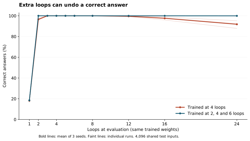

At 24 loops, two mixed-depth runs still had all 4,096 answers correct. The other missed seven. We hadn't trained any of them beyond six loops. Varying the stopping point had made this little model much less likely to lose its answer when we extended the computation.

This wasn't a new failure mode waiting to be named. Loop, Think, & Generalize studies recurrent-depth models and describes degradation under excessive recurrence. [2] The useful part of building a small version was seeing how much the result changed with the training schedule. Our first curve, by itself, would have made continued looping look much less promising than the second one did.

Six hops still finished too quickly

We next asked for the whole six-hop path through a sixteen-node graph. Getting five positions right and one wrong counted as a wrong answer. The models trained at a fixed six loops all reached at least 99.4% complete-path accuracy there. At 64 loops, their scores were 8.79%, 64.50% and 1.46%.

That looked like a much bigger penalty for a longer answer, but individual hops survived better than complete paths. One changed position is enough to spoil the latter. The two panels below show both measurements; looking only at complete-answer accuracy makes the collapse look more comprehensive than it is.

This still didn't address the case we wanted most: a model that needs dozens of iterations to arrive at an answer in the first place. Some of these six-hop models solved the task in three or four passes. Their attention could see the whole graph; the number of links wasn't a reliable measure of how many loops they needed.

A task that cannot finish in six loops

For that test, we changed how information could move. Each node could attend only to itself and its next neighbour. We put a random 16-bit payload at one end of a chain and asked the other end to recover it. Across 32 links, information about that payload cannot arrive before the 32nd pass.

That lower bound comes from the attention restriction we imposed. This is a controlled test of carrying and preserving information through repeated computation; copying the payload doesn't become a difficult reasoning problem merely because we made the chain long. The restriction does let us rule out an answer obtained through a global-attention shortcut.

Getting even that to work took a few attempts. Starting directly at 32 links left the model near guessing. A curriculum learned short chains but struggled as they grew. We then normalized the state after each residual update and trained through chains of 4, 8, 16 and 32 links, allowing two loops per link. The last stage therefore read the answer at loop 64.

We kept 512 distinct payloads out of training and evaluated the same checkpoints out to 256 loops. Once the coarse sweep showed a peak, we went back and sampled every loop from 32 to 96. No weights changed during that closer look.

$ python dense_report.py
32 links / 16-bit answer / 512 held-out payloads
Same checkpoints; evaluation sampled one loop at a time

seed   best loop   complete answers    at 64    at 80
  11          64       50/512           50        2
  22          61        2/512            2        1
  33          64      406/512          406        6

The third seed recovered 406 of the 512 complete answers at loop 64. The other two recovered 50 and 2. That difference matters: the training wasn't reliably solving the long task across runs. But in the run that learned it best, we could finally watch an answer arrive after dozens of passes and then disappear.

Two more loops were enough to lose a bit

The following is the first payload in seed 33 that was correct at loop 64 and wrong at loop 80. All sixteen bits have to match. We included the earlier attempts as well as the correct answer; you can see it getting closer before it reaches the target.

Seed 33 / item 0
expected 1000000110000000
loops    predicted answer  correct bits
   48    0010100110000010   12/16
   56    1000000110000110   14/16
   60    1000000010000100   14/16
   62    1000000110000100   15/16
   64    1000000110000000   16/16
   66    1000000110000010   15/16
   68    1000001110000010   14/16
   72    1010001110000010   13/16
   80    1010001110000010   13/16
   96    1010001110000010   13/16

At 62 loops, one bit is still wrong. At 64, they all match. At 66, a different bit has changed. Nothing new entered the model between those readings. We simply applied its block again.

Across the full test set, that seed fell from 406 correct answers at loop 64 to six at loop 80. By 96, none were completely correct. Individual examples can deteriorate a bit at a time while the complete-answer score falls sharply; a single flipped bit removes an example from that score.

The location of the peak is hard to miss. Sixty-four loops was also the stopping point used in the last training stage. We had trained the model to deliver an answer there. We had not required the answer to remain usable indefinitely afterwards.

Trying to widen the window

Changing the training depths had helped the first, smaller model. We tried a related change here: another 1,200 updates, this time supervising nodes that could have received the payload at several intermediate loops. The idea was to make a correct representation useful at more than the final stopping point.

It wasn't a successful fix. In seed 33, complete-answer accuracy at loop 64 fell from 79.3% to 8.2%. At loop 128 it improved from zero to 5.7%. We had kept a few answers alive longer while losing most of the strong result at the original stopping point. The other seeds remained weak.

$ python refinement_report.py
32 links / complete 16-bit answers, percent correct
Extra training also changed the supervision objective.

seed stage          64      80     128     256
  11 before     9.77    0.39    0.00    0.00
  11 after      0.98    1.17    0.78    0.39
  22 before     0.39    0.20    0.00    0.00
  22 after      2.15    1.76    0.20    0.00
  33 before    79.30    1.17    0.00    0.00
  33 after      8.20    8.01    5.66    0.78

We changed the objective as well as adding training, so this comparison can't isolate either one's effect. What it does show is that the promising result from varying depths on the small task wasn't a ready-made solution for the longer one.

Astra is the larger-scale connection that prompted the experiment, and this gives us a specific behaviour to wonder about there: an answer can become correct during recurrent computation and then be lost. Here we could see the last missing bit arrive at loop 64. We haven't yet found a training setup that reliably lets the following passes preserve the whole answer.

What does this mean?

There’s a sweet spot in how long you let the model work. A simple question may be answered early, leaving later iterations to disturb something that was already correct. A complex question needs more passes; stop too soon and you get an answer that the model could still have improved.

You can see both sides in the bit trace. At 62 loops, the answer wasn’t finished. At 64, it was correct. At 66, it was wrong again. The useful stopping point sat between unfinished work and a result that had started to deteriorate.

That makes deciding when to stop part of solving the problem. A fixed loop budget has to serve questions of different difficulty. An adaptive one has to recognise when further computation is helping, and when it should leave the answer alone.